Dress in Layers
Convolutional neural networks (CNNs) improve on our ability to extract predictive features from image data, allowing us to classify image objects with greater accuracy. Here I will walk through some of the underlying principles of regular and convolutional neural networks, and then demonstrate the construction of a CNN in Keras, which I have iteratively tweaked, with the goal of categorizing images of fashion items into appropriate classes with a high degree of accuracy.
CONTENTS:
- The Fashion-MNIST Data Set
- Random Forest, GradientBoosting and SVC: Reproducing Results
- Import Packages and Preprocessing
- Neural Networks: A Primer
- Convolutional Neural Networks and Image Data
- >0.93 Accuracy on Fashion-MNIST with CNN in Keras
- Visualizing the CNN Training Process
- Model Summary
- Where Does the Model Make Mistakes?
- Additional Directions
The Fashion-MNIST Data Set
One of the classic benchmark data sets for testing the effectiveness of neural network architectures at image recognition tasks is the MNIST data set. This is a large database of 28x28 grayscale images of handwritten digits collected from Census Bureau employees and high school students. The digits are size-normalized and centered in a fixed image. The goal is to train a neural network on the larger training portion of the data set, and then test how accurately it categorizes digits from the smaller test portion of the dataset. This data set has been in use since the late 1990s, and is the most widely referenced database in machine learning image analysis.
In recent years, the original MNIST data set has become dated. The primary problem is that it is too easy, with neural net models able to achieve upwards of 99.7% accuracy, and even classic machine learning algorithms able to break 97%. It is also overused, and fails to represent the real-world complexity of modern computer vision tasks.
The Fashion-MNIST Data Set, created by researchers at the e-commerce company Zalando, is intended as an MNIST replacement, for use in benchmarking machine learning algorithms in image analysis. Fashion-MNIST mirrors MNIST in structure and format. It contains 70,000 28x28 pixel grayscale images of fashion articles in 10 categories, similar to the 10 digits in MNIST. The training set contains 60,000 images (6000 from each category) and the test set 10,000 images (1000 from each category). The categories are listed and visualized (three rows to a category) in the image below.
![]()
The advantages of Fashion-MNIST are that it is significantly more challenging (see below) than MNIST, and provides a better model for real-world computer vision problems. It is seeing increasing adoption over MNIST, and has recently been added as a standard data set in Keras.
When working with Fashion-MNIST, the feature variables will be the grayscale values for each of the 784 pixels in a given image, loaded either as a 784x1 vector or as a 28x28 array. The target variable is a number from 0 to 9 (inclusive), representing which of the 10 categories the pictured fashion item belongs to. The challenge of course is how accurately can we classify images in the test set into their true categories, based on what we learn from the training set.
Random Forest, GradientBoosting and SVC: Reproducing Results
Below is a list of benchmarks by established sklearn machine learning classifiers, with different hyperparameter combinations, for the Fashion MNIST dataset. They are listed in order of highest mean accuracy on test data. I was able to reproduce results for the Random Forest and Support Vector classifiers, the others were time prohibitive.
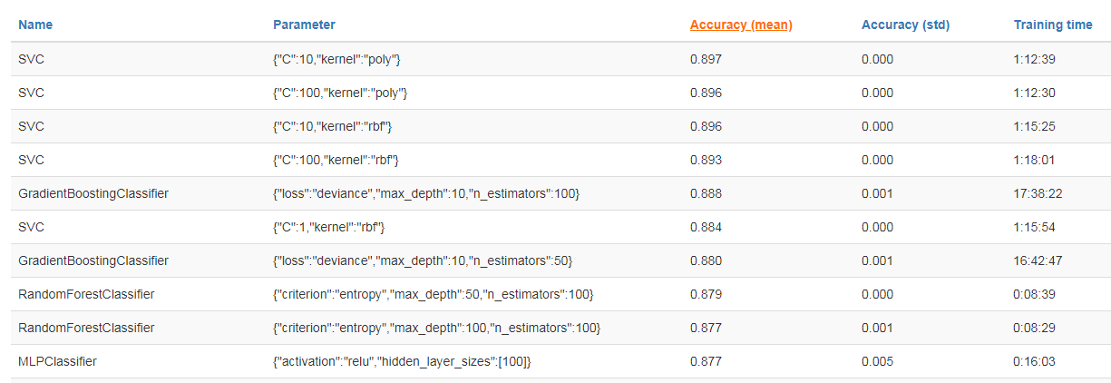
These performance benchmarks in the 0.85 to 0.90 range can be considered a baseline for us. We will try to improve upon these with specialized and tuned neural networks.
Import Packages
#Import standard packages
import pandas as pd
import numpy as np
import matplotlib.pyplot as plt

#Import Keras packages for neural network design
from keras.models import Sequential
from keras.layers import Dense, Input, Dropout, Activation, Flatten
from keras.layers import Conv2D, MaxPooling2D, BatchNormalization
from keras.utils import np_utils
from keras.callbacks import EarlyStopping, ModelCheckpoint, LearningRateScheduler
from keras.models import load_model
from keras import regularizers

#Load the Fashion-MNIST Data Set
from keras.datasets import fashion_mnist
(x_train, y_train), (x_test, y_test) = fashion_mnist.load_data()
Preprocessing
#Set a random seed for reproducibility.
np.random.seed(42)

#Load in the Fashion MNIST data set.
from keras.datasets import fashion_mnist
(x_train, y_train), (x_test, y_test) = fashion_mnist.load_data()

#Reshape the data to have depth of 1.
x_train = x_train.reshape(x_train.shape[0], 28, 28, 1)
x_test = x_test.reshape(x_test.shape[0], 28, 28, 1)

#Grayscale values run from 0 to 256.  This scales that data to a 0 to 1 range and converts to float.
#Perhaps unnecessary with Fashion MNIST, but scaling like this is best practice with image data.
#It also may improve computation efficiency.
x_train = x_train/255.
x_test = x_test/255.

#The target variable needs to be one-hot encoded, i.e.; converted into a purely categorical form.
#Leaving it as 0-9 would create false proximity relationships between the categories.
y_train = np_utils.to_categorical(y_train,10)
y_test = np_utils.to_categorical(y_test,10)
Neural Networks: A Primer
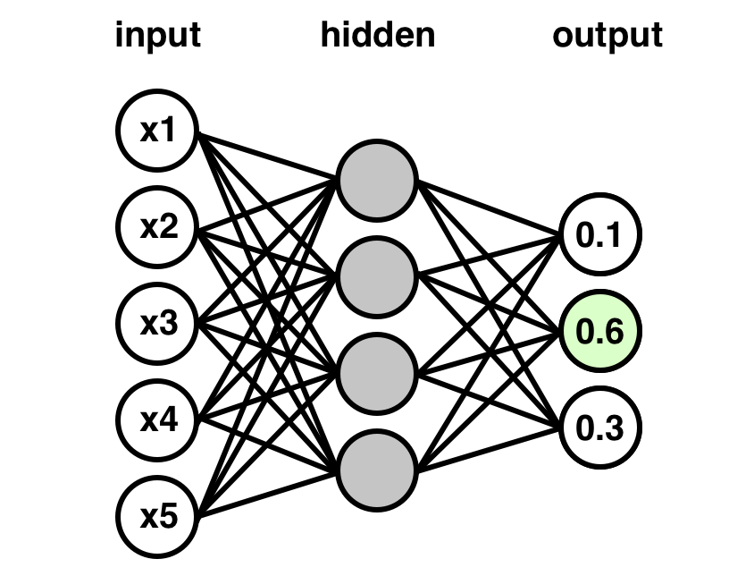
Regular neural networks are composed of sequential layers, and work roughly as follows:
- Data is fed into an input layer of neurons, typically in the shape of the data itself.
- The data is fed forward through one or more hidden layers, of a chosen size. We can think of these hidden layers, loosely speaking, as controlling particular intermidate features of the data, for example initial layers might have nodes corresponding to small feature fragments, and larger, composite features that could potentially classify an image handled in later layers.
- A final output layer consists of one neuron for each class designation (10 in this case), one of which is activated by the final calculus of the network based on an individual input.
- Every neuron in the network starts with a weight and bias with which it transforms incoming data. Most often these are initialized arbitrarily. The input data for a given individual is fed into this system of interlocking weights and biases and generates a classification decision, mathematically, for that individual. Basically, the data from the previous layer is transformed by each neuron's weight and bias and returns a value for that neuron that determines whether it is activated or not, with only activated neurons influencing the next layer. This results in each output layer neuron ending up with a predicted probability, the highest of which will be the predicted class.
- After a certain number of individuals in the training data (called a batch) have been fed through the system this way, the neural net compares its classification predictions (more accurately, it's prediction probabilities) to the true class values (1 for the correct answer, 0 for everything else). The neural net than backpropagates, adjusting the weights and biases of each neuron so as to minimize its predictive error relative to the correct values. Different loss functions can be minimized depending on the purpose of the network, in this case we will minimize categorical cross-entropy, a loss function designed for multi-class classification, with especially strong penalties for confidently incorrect predictions.
- After the network has tweaked itself, the next batch of individuals from the training set is fed into the system with the newly calibrated weights and biases at each node, generating (theoretically) better classifications. After each new batch is fed through, the system backpropagates again to adjust its characteristics before proceeding, continuing like this until it has fed through the entire training set. This concludes one epoch. The network typically returns a validation score on the test set at this time, then begins running through the training data again to improve itself further.
- Some networks will train over hundreds of epochs. However there also comes a point where the network will begin over-training to the data, which will eventually start to reduce validation accuracy.
I started out using simple sequential neural networks like this in Keras, and was able to outperform sklearn benchmarks after only a few short training epochs. Validation accuracy topped out just over 0.89. To increase performance, I turned to the gold standard in machine learning image classification: the convolutional neural network (CNN).
Convolutional Neural Networks and Image Data
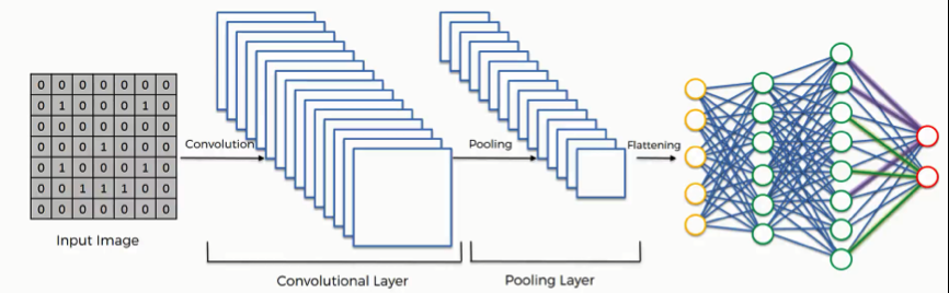
With convolutional neural networks, we add specialized layers to the front end of our sequential neural network that help to identify image features, while also creating condensed image representations that reduce the number of parameters our dense sequential layers will need to process. This parameter reduction improves learning efficiency and greatly reduces our risk of overfitting. Because of the nature of image data, we can often condense pixel values without losing meaningful information about the image, and in fact, the condensed representations are often cleaner mathematical representations of the features in an image than the larger, more complex originals. The specialized layers that we add will consist primarily of convolutional layers, followed by one or more pooling layers, and then a flatten effect that will reduce the data to a format that can be fed into the dense sequential layers of the network.
The convolutional layers come first, and essentially apply a series of numerical filters to each image which convolve the image, meaning that we pass the filter across the image in steps, filtering down sections of pixels into single values by calculating the dot product of the filter and the image segment. These layers may condense the data slightly, depending on the options we set, but their primary purpose is to transform the data from raw pixel values into relational values that describe how pixels near each other compare and contrast. This allows for rudimentary image comprehension.
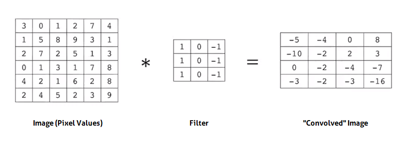 Different filters can be designed to identify different features of an image (e.g.; vertical edges, pictured above), depending on the numerical composition of the filter. But we don't specify anything here; rather, we allow the network to design the filters itself, by trial and error. When we create convolutional filter layers, the filters within them are instantiated with random values, which are then updated to improve performance during the fitting process, when the model backpropagates - much like the weights and biases of neurons in regular, densely connected sequential layers. In this way, the convolutional layers of the network eventually learn to filter the images for whatever features have the most predictive value.
The weights for each filter in the convolutional layer are additional parameters that the model will have to optimize. However, this is a small tradeoff for the large number of parameters excluded by filtering images down to condensed representations. More importantly perhaps, the target-driven feature identification provides a powerful interpretive step toward image classification.
There are multiple options (a.k.a.; hyperparameters) that can be set for convolutional layers. A very clear and helpful visualization of the convolution process and some of the hyperparameters involved can be found here.
Pooling
I've talked about how convolutional neural networks reduce the number of parameters in our model. The majority of this reduction occurs not in the convolutional layers themselves, but in the subsequent pooling layers. As the name suggests, pooling layers pool groups of neighboring pixels into a single value.
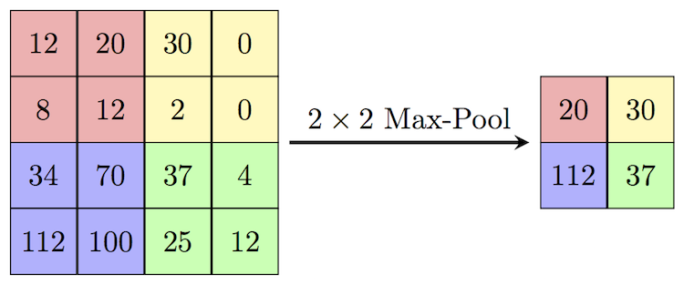
Recall that convolutional layers pass a sliding filter over each image and produce a set of relational values that represent features in the image. We now take those outputs and apply a pooling filter to them. Unlike the convolutional filter, the pooling filter does not slide across the image. If the pooling filter is 2x2, the image is subdivided into distinct 2x2 partitions and the pooling filter reduces each partition to a single value. In the standard pooling method, max pooling, that single value is simply the maximum value in the pool. So in our example, the max value is taken forward from each 2x2 group of pixels, and the rest of the values dropped. See below.
This process typically allows us to greatly reduce the feature complexity that the network has to handle, while more or less preserving the feature extraction performed by the convolutional layers. Some CNNs will have pooling after each convolutional layer, while others will have pooling only at the end of convolution. After convolution and pooling are complete, the final output is flattened into one dimension and fed into the dense sequential layer portion of the network.
>0.93 Accuracy on Fashion-MNIST with CNN in Keras
I went through a number of iterations, trying to find the most effective components, preserving tweaks that saw clear gains and combining different strategies in ways that seemed sensible. The following model provided the best performance.
Structure
After initializing our network in the first line, we begin with four convolutional layers. We use Conv2D because the data we are operating on is 2-dimensional. Using a series of convolutional layers is advisable in general in image analysis, as it allows the system to develop tiered feature detection. For instance, a first convolutional layer might end up detecting raw edges, while the second uses these edges to detect simple shapes, and a third detects higher level features in these shapes that contribute well to classification. The kernel size hyperparameter controls the pixel dimensions of the filters in each layer, i.e.; the sliding window we pass over the image. For images that are only 28x28 to begin with, 3x3 is a sensible filter size. We have also added padding, which means we create empty space around each image so that the filter can pass over every part of the image an equal number of times, rather than undersampling the edges and corners.
After the convolutional layers I ended up with a single max-pooling layer. The pool size hyperparameter controls the dimension of the pools, in this case I have used 2x2. I suspect the effectiveness of just the single pooling layer with a small pool size is due to the small size of the images to begin with (28x28). Any more pooling on that, and we're probably just introducing bias. Even an image of, say, 200x200, would probably benefit from more extensive pooling than what we have here.
After pooling and flattening, I have added a single dense layer of 128 neurons, followed by a 10 neuron output layer representing the classification output. The final classifying layer uses the softmax activation function, which converts the vector it receives from the final hidden layer into a probability distribution that sums to 1. The highest probability will correspond to the model's class prediction. All preceding layers are set to use the standard relu activation, or rectified linear units. This function simply converts any negative neuron outputs to 0, while feeding all positive values forward. When we speak of neurons in a layer being activated or not for a particular image, this is what we mean - we have some activation criteria (the most common is simply >0), and if activation criteria are not met by the neuron's output value, then the neuron is reduced to 0 (inactive), so that its mathematical effect is null.
Batch Normalization
This is the basic structure of the network. But we can also interpose Keras layers that are not actual structural layers of nodes, but rather ways of manipulating the node layers to increase the effectiveness of the network. The first such layer that we've used here is a normalization layer called BatchNormalization. Batch normalization is a technique introduced in a 2015 paper in which we normalize the activation output of the prior layer, basically scaling the outputs so that they have approximately mean 0 and standard deviation 1. As the name suggests, this is done on the batch interval, so concurrent with each backpropagation. Empirically, batch normalization broadly improves performance, as well as learning speed, and I certainly saw gains after applying it. It is possible to apply batch normalization to all hidden layers in a network; but it's also common to apply it only to the input layer, which I have done here.
Dropout
The other major manipulative layer type that we will use is Dropout. Dropout is a very effective regularization technique that reduces overfitting and improves generalizability when training deep neural networks. When applied to a neuron layer, it randomly drops out a specified percentage of the neurons in that layer over each training epoch during the training process, essentially clearing the influence of those nodes on the model's predictive process for one epoch, allowing other nodes to compensate for their missing influence, before eventually reinstating the dropped neurons and dropping some other subset as training continues. The effect of this technique is similar to training multiple neural networks that have the same structure, in parallel, and averaging their predictions - but with far less compute. By excluding neurons from periods of the training process, Dropout is able to break up situations where layers are compensating in complicated ways for "mistakes" in a previous layer. The result of Dropout is a model that is more robust and more resistant to early overfitting.
Employing Dropout on the pooling layer output and the dense hidden layer clearly and immediately improved how long my model could train without overfitting, as well as its final performance. I saw particular gains again when I added a modest dropout rate to the convolutional layers themselves. This is when my model began to approach test accuracy around 0.93.
The low to moderate dropout rates that I've used in this network were the most successful over a relatively short training period. However, it is possible that we could see even higher accuracy from the model if we employ substantially higher dropout rates (0.5 to 0.8) and simply train for much longer.
Fitting the Model
Finally, we compile and fit the model. As discussed earlier, the loss function here will be categorical cross-entropy, and our metric is accuracy score, i.e.; the percentage of test set images that the model predicts correctly. The batch size I've used here is 128, meaning that during training, backpropagation to update parameters occurs in the network after every 128 images. I've run the model for 20 epochs in this case. In other instances I trained longer, but 20 epochs is all that is required to reach the start of overfitting in this model.
The last thing worth mentioning is that prior to fitting I have included a ModelCheckpoint. This is a very handy Keras feature that can be used to save the model state at the end of each epoch, or in this case, to save whichever end-of-epoch model state has the highest validation accuracy. This prevents us having to worry about timing the model to end prior to overfitting. We can simply access the peak performance model state automatically in the loadable .h5 file that ModelCheckpoint creates.
The full model training is below:
#The top-performing convolutional neural network structure (Accuracy > 0.93)
cnn = Sequential()
cnn.add(Conv2D(32, kernel_size=3, activation='relu', input_shape=(28,28,1),padding='same'))
cnn.add(BatchNormalization())
cnn.add(Dropout(0.2))
cnn.add(Conv2D(32, kernel_size=3, activation='relu',padding='same'))
cnn.add(Dropout(0.2))
cnn.add(Conv2D(24, kernel_size=3, activation='relu',padding='same'))
cnn.add(Dropout(0.2))
cnn.add(Conv2D(64, kernel_size=3, activation='relu',padding='same'))
cnn.add(MaxPooling2D(pool_size=(2,2)))
cnn.add(Dropout(0.2))
cnn.add(Flatten())
cnn.add(Dense(128, activation='relu'))
cnn.add(Dropout(0.3))
cnn.add(Dense(10, activation='softmax'))

cnn.compile(optimizer='adam', metrics=['accuracy'], loss='categorical_crossentropy')

#ModelCheckpoint allows us to extract the best end-of-epoch model.
#Under different circumstances, we might monitor validation loss instead of validation accuracy.
callback_list=[ModelCheckpoint(filepath='cnn.h5', monitor='val_acc', save_best_only=True, mode='max')]

cnn.fit(x_train,y_train,validation_data=(x_test,y_test),batch_size=128,epochs=20,verbose=1,callbacks=callback_list)
Visualizing the CNN Training Process
The function below plots improvement in validation accuracy over the course of training (left), and loss reduction over the course of training for both the training data and test data. This model performs quite well, with loss dipping below 0.21, and testing loss tracking well with training loss over time. Training loss will continue to improve indefinitely, as the network works to minimize it further and further. The point at which training loss becomes lower than testing loss is where the model is starting to overfit. However, there may still be slight improvements in validation loss beyond this point.
def accuracy_loss_plots(model):
    fig, (ax1,ax2) = plt.subplots(nrows=1,ncols=2,figsize=(12,5))
    ax1.plot(model.history.history['val_acc'])
    ax1.set_title('Test Accuracy by Epoch')
    ax1.set_xlabel('Epoch')
    ax1.set_ylim(0.8,1)
    ax2.plot(model.history.history['loss'], label='Training loss')
    ax2.plot(model.history.history['val_loss'], label='Testing loss')
    ax2.set_title('Loss Reduction by Epoch')
    ax2.set_xlabel('Epoch')
    ax2.set_ylim(0,1)
    ax2.legend();
accuracy_loss_plots(cnn)

Model Summary
After loading in the best model state saved by ModelCheckpoint, we can confirm the validation loss and validation accuracy, and look at a summary of the structure and parameter count in the model, as well as the progressive output shape from each layer.
#Load in the best model state from ModelCheckpoint
cnn_best = load_model('cnn.h5')
#Confirm loss and accuracy on the test data
cnn_best.evaluate(x_test,y_test)
cnn_best.summary()
Where Does the Model Make Mistakes?
We can generate a multi-class confusion matrix to identify where our model is error-prone, and in particular, which fashion categories the model struggles to distinguish.
from sklearn.metrics import confusion_matrix
from itertools import product

classes = ['T-shirt/Top','Trouser','Pullover','Dress','Coat','Sandal','Shirt','Sneaker','Bag','Ankle Boot']

#Create Multiclass Confusion Matrix

preds = cnn_best.predict(x_test)
cm = confusion_matrix(np.argmax(y_test,axis=1), np.argmax(preds,axis=1))

plt.figure(figsize=(8,8))
plt.imshow(cm,cmap=plt.cm.Reds)
plt.title('Fashion MNIST Confusion Matrix - CNN')
plt.colorbar()
plt.xticks(np.arange(10), classes, rotation=90)
plt.yticks(np.arange(10), classes)

for i, j in product(range(cm.shape[0]), range(cm.shape[1])):
    plt.text(j, i, cm[i, j],
    horizontalalignment="center",
    color="white" if cm[i, j] > 500 else "black")

plt.tight_layout()
plt.ylabel('True label')
plt.xlabel('Predicted label');

Here we can see how many individuals in each class have been predicted to their correct class, versus predicted to some other class. Immediately it is clear that there are certain categories that cause most of the error in the model. The categories "Shirt", "T-shirt/Top", "Coat", "Pullover", and "Dress" - basically anything in the shape of a top - create the majority of confusion. "Sneaker", "Ankle Boot" and "Sandal" are also mixed up on occasion. These results are encouraging. They indicate that the convolutional layers have zeroed in on features that have meaning: categories with similar shape features are occasionally being confused, while more distinct categories are pretty much not.
One approach that would be an interesting direction here would be to establish a sort of hierarchical neural network system. So, perhaps a first network which classifies into one of four groups: tops, footwear, bags, trousers; and then separate networks that train to discriminate between the finer classes that compose the tops and footwear groups, rather than asking a network to train on these differently resolved class distinctions all at once.
Additional Directions
In addition to this hierarchical networks concept, we discussed earlier that higher dropout rates combined with larger numbers of nodes and longer training, could potentially yield higher accuracy. We could also consider BatchNormalizing at every layer. We could also experiment with data augmentation, which would consist of generating slightly rotated versions of the images in the training set to produce a much larger training set, and potentially a more robust model overall.
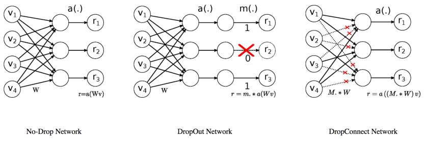
Another approach that might be useful involves a recent, interesting innovation on the Dropout concept called DropConnect. Rather than dropping out a certain randomly selected percentage of neurons in a layer for each training epoch, DropConnect drops out a randomly selected percentage of neuron weights, in a sense creating a more finely optimizable version of the Dropout effect.
Perhaps the most famous use case of DropConnect is its involvement in the current highest reported legitimate accuracy on the original MNIST data set (99.79%). So there's reason to believe it could be helpful here as well. I was able to locate a Keras implementation of DropConnect and get it working. DropConnect can be run in tandem with regular Dropout, however it only works on dense hidden layers, of which I only had one in my model. Therefore, while the model performed just fine with DropConnect employed, it didn't move the needle in terms of test accuracy. The question is, if we were training a deeper network with higher Dropout rates as suggested above, and perhaps multiple densely connected layers, might we start to see more value from DropConnect.